Taking a “latent variable” approach to modelling bernoulli probabilities using maximum likelihood estimation and the logit link function.
A latent variable model
Imagine a basketball player is taking free throws.
For each trial \(i\) (a freethrow attempt), we observe the outcome \(y_i\) as being 1 if there is a success (i.e. the freethrow is made), or 0 if it is a failure (a miss).
When the player takes the freethrow, there are exogenous features \(X_i\) that influence their likelihood of making it (e.g. whether they are home or away). Also there is some randomness, \(\varepsilon_i\) that is unpredictable: a 99% accurate shooter still has a 1% chance of missing.
Economists often frame this problem as a “latent variable model”. What this means is they frame the problem as though there is a hidden continuous variable we do not observe, \(y_i^*\), and if it exceeds a certain threshold (usually zero) then there is a success (e.g. the freethrow is made):
In other words, the latent variable \(y_i^*\) is purely a function of its predictors \(X_i\), their relationship to \(y_i^*\) given by \(\beta\), and some additive noise \(\varepsilon_i\). If \(y_i^*\) is positive, we observe a success (i.e. \(y_i = 1\)).
We can thus formulate the probability of success \(P(y_i=1|X)\) as the likelihood that the additive noise \(\varepsilon_i\) is less than \(X\beta\), resulting in the probability \(y_i^*\) above zero:
So a good assumption for the probabilistic process that generates the error \(\varepsilon_i\) is very important! We will come back to this shortly, after discussing the Bernoulli probability mass function.
The Bernoulli PMF
Even if a player has a 99% of making freethrows, they would be expected to miss 1 in 100. We can capture this through the probability mass function of the Bernoulli distribution:
Until now, we have just been looking at the likelihood of making a success for a single trial \(i\). But we want to find values for \(\beta\) that optimize predictions across all trials, to learn the impact of \(X\) so we can better predict \(y\) next time - aka maximum likelihood estimation.
Maximum Likelihood Estimation
Assuming each trial is independent (a big assumption for free throws!) - the probability of making two then missing one is \(p_i \times p_i \ \times (1-p_i)\). In other words - the combined probability is the multiplication of the individual probabilities.
We can generalize this to a sample size \(N\) as the following:
In practice, it is common to minimize the negative log-likelihood, which is shown to be equivalent to maximising the likelihood directly (since the logarithm is a monotonic function):
Recall that \(\log{\left(ab\right)} = \log{\left(a\right)} + \log{\left(b\right)}\)
We now - almost - have a well defined problem we can solve! We just need to make an assumption for the distribution of errors \(\varepsilon\).
Assuming errors come from a logistic distribution
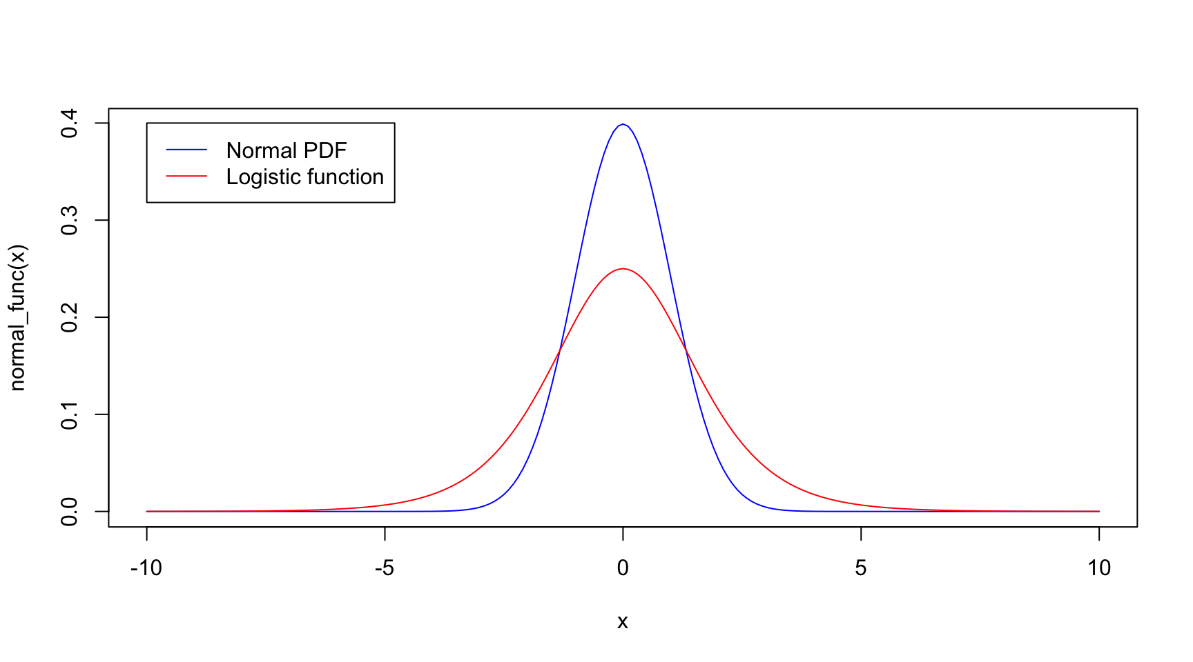
The errors are often assumed to be generated from a logistic distribution, with location parameter \(\mu=0\) and scale parameter \(s=1\):
\[
\epsilon \sim \text{Logistic}(0,1)
\]
Why a logistic? Well because is highly similar to a normal distribution, but with fatter tails, so its seen as an approximation that is more robust. Furthermore, it has easier algebra to unpick - which we will show shortly.
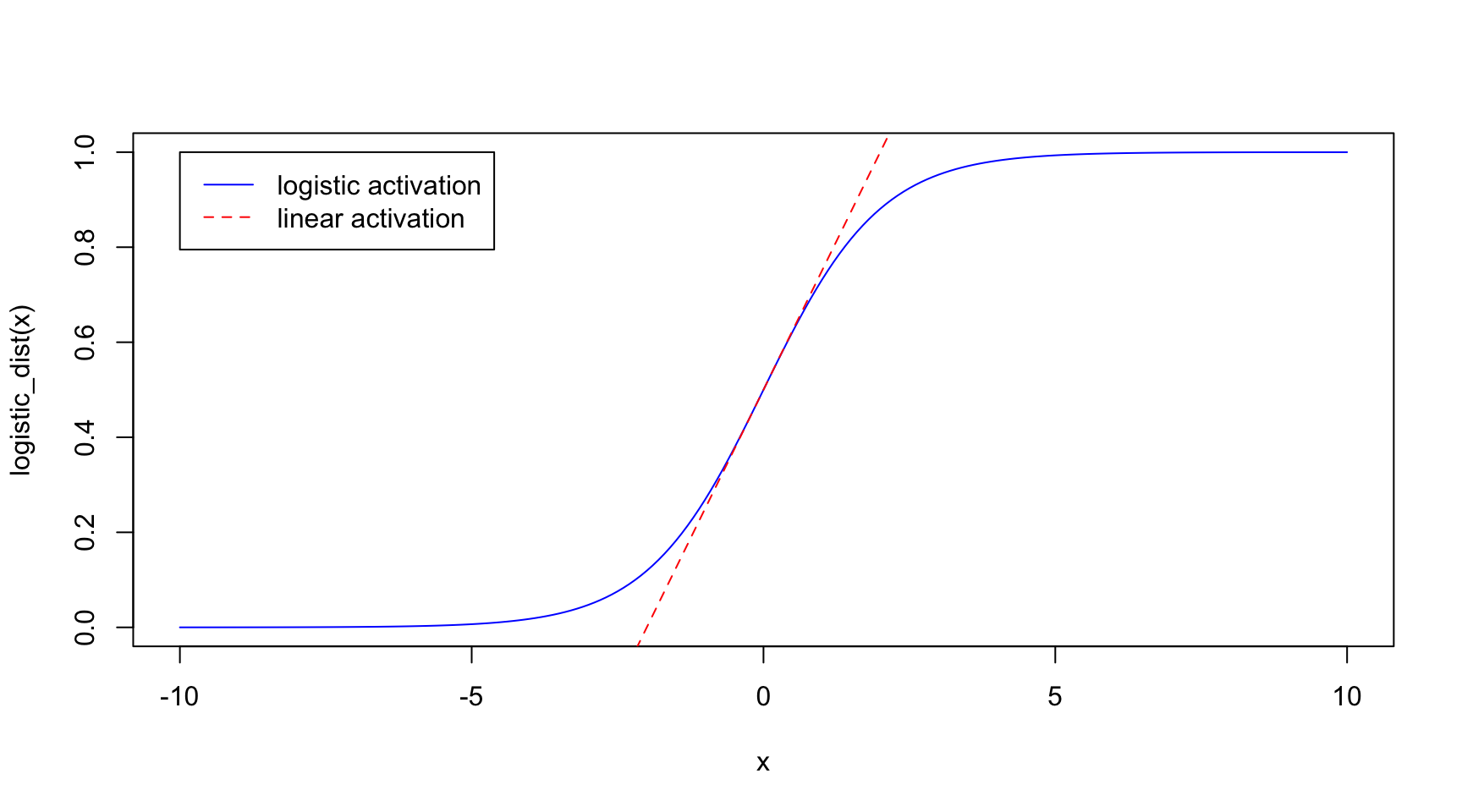
For probabilities of between 0.3 to 0.7, we see that the logistic activation function maps very closely to that of a simply linear one. It is only at the more extreme probabilities that they diverge.
Linearity in terms of log-odds!
To further intuition, it can also be useful to rearrange the regression in terms of \(X_i\beta\).
By doing this, we find that we are fitting a model where the “log-odds” are linearly related to its predictors:
Log-odds means taking the logarithm of the probability of success divided by the probability of failure
This is a “link function” - the link between the outcome, \(y\), and the linear predictors \(X\) via \(\beta\). This specific link function is called the “logit function”.
And so it is now clear the inverse logit is the logistic function:
This is as far as we can get without modelling \(P(\varepsilon_i < X \beta)\). So let’s look at substituting \(p_i\), \(1-p_i\), \(\partial p_i/\partial \beta\) and \(\partial (1-p_i)/\partial \beta\) into our first moment condition to derive the optimal coefficients:
Thus there is no closed form solution like OLS. However, given the cost function is convex, using an optimization like Newton Raphson will find the optimum coefficients.